
Part 2
Previously on Dr. Reproducible Research
In the previous part of this article, I explained the reasons and motivation behind my attempt to revisit one of my PhD papers and try to:
- Reproduce it from the text.
- Rewrite the code in Python instead of Matlab.
- Reproduce the results from the original paper.
- Try to reproduce results on KITTI, as reported by a newer paper.
Examining the essence of a scientific paper
My original paper was called “Random-Walker Monocular Road Detection in Adverse Conditions Using Automated Spatiotemporal Seed Selection” and it can be downloaded from here, for people with IEEE access. At the time of writing this piece, it had 24 citations as reported by Google Scholar.
My first thought when I started re-reading my own work, was the unfortunate selection of the word “detection”, instead of the more proper “segmentation”. Oh well… there are so many other things to complain about, that I am going to let this one slide.
The objective of the paper was to demonstrate an algorithm that robustly detected the driveable road area in front of a moving car, using as only input the video stream of an on-board monocular camera. A quantitative demonstration of the results was performed on the DIPLODOC sequence and a while later I added 2 videos from Jose Alvarez’s work. For qualitative analysis I used several videos captured with an experimental setup of 4 cameras and an AVerDiGi recorder that we had fixed on my advisors car :)
The final proposed system (which is the focus of this article), was pretty simple to describe in just a handful of steps:
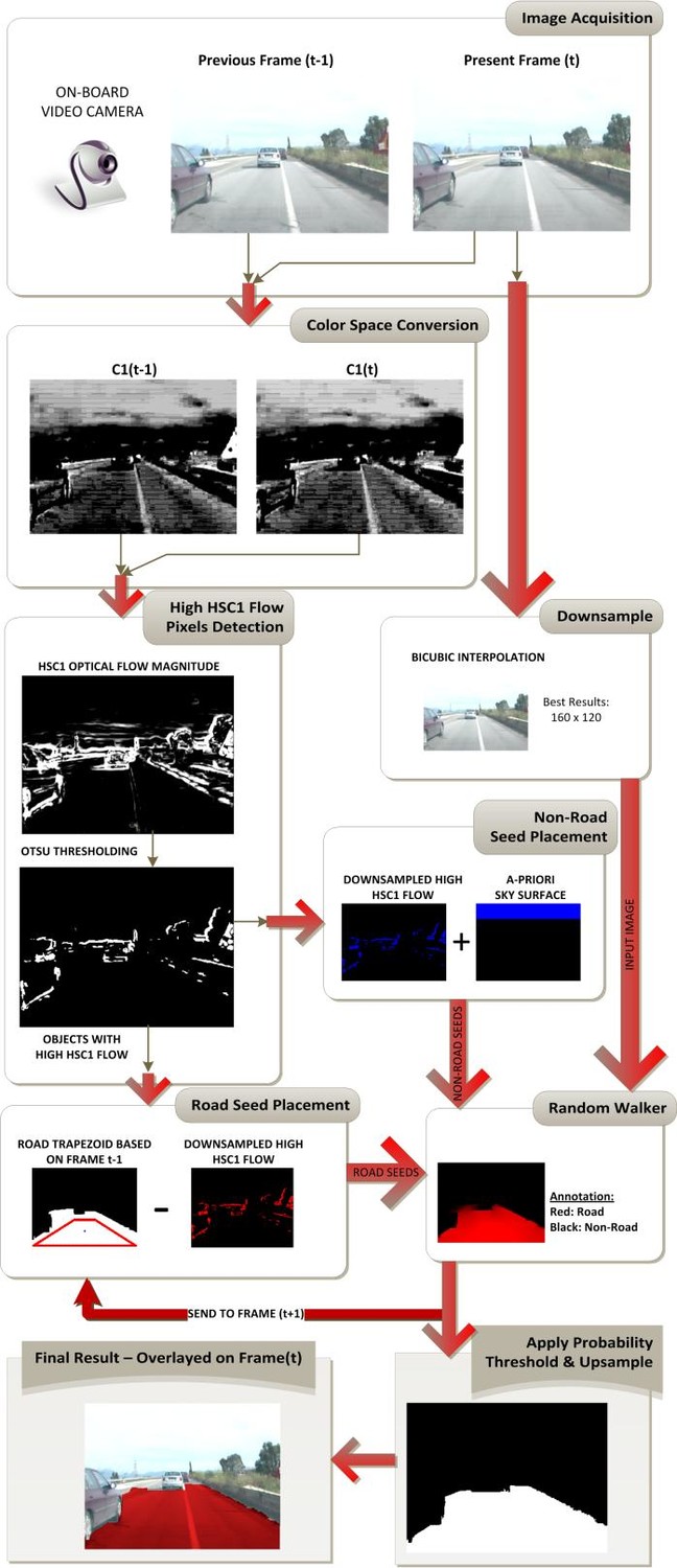
- Get a pair of consecutive frames from the video.
- Keep the second frame to perform the road detection process and downsample it to 120x160 for better performance and less noise.
- Convert both images to the C1 channel of the C1C2C3 color space. More details on this exist in the paper, but for completeness, at each pixel coordinate x, y of the image: C1(x, y) = arctan(R(x, y) / max(B(x, y), G(x, y))).
- Perform Horn -Schunck Optical Flow on the results of (3). Call this HSC1 so that it is not mistaken for classical optical flow.
- Use Otsu’s thresholding method to threshold the magnitude of HSC1.
- High HSC1 values from (5) and an area in the top of the image are assigned the label “non-road”.
- The perimeter of a trapezoidal area in front of the car is assigned the label “road”, except the pixels of the perimeter with a high HSC1 value.
- The labels from (6) and (7) and the image from (2) are fed as seeds into a Random Walker image segmentation algorithm.
- The pixels with probabilities above 0.5 (due to the 2-class problem we are solving) to belong to the road, are labeled as “road”.
- The result of (9) is used to initialize the “road” seeds of the next frame more accurately.
- The result of (9) is upsampled to the original resolution and used to calculate the performance metrics for the given frame, when of course we have the ground truth for it.
- The only thing remaining, are the optimal parameters, as proposed in the paper. For HSC1 calculation, the parameters are a = 3 and iterations = 1. For random walker, the only parameter needed is: beta = 90.
Picking up the ingredients
With these 11 steps and the ideal parameters in mind, we can go ahead and search for the necessary Python modules that will allow us to rapidly reproduce the results.
- The first thing we need, is a module that allows for image I/O and as many basic manipulations as possible. We could go for OpenCV, but it would be an overkill and we could be even more Pythonic in this exercise. Also, we would like to be closer to Matlab style, to be able to compare the methods easier. For this reason, I chose scikit-image.
- For general array manipulations, indexing and code vectorization to be possible, of course numpy.
- For visualization, matplotlib and for easy streaming visualization at runtime (optional), drawnow.
- For file reading, directory content lists etc, os from native Python.
- For optical flow, there is a handy module named pyoptflow.
- For Otsu’s thresholding method, scikit-image provides an implementation in filters.
- For basic processing time monitoring and logging (optional), time and logging from native Python will be used (I love it when things are so obvious).
- For nice process bars (optional), tqdm.
- Bonus track: the most difficult and tricky part is random walker. This is included in scikit-image. For performance, we should also install pyamg, numexpr and scikit-umfpack.
- A nice-to-have couple of modules that may come in handy, are also scikit-learn and scipy.
- Finally, jupyter for using ipython and jupyter notebooks. Also, (optional) jupyterlab.
Concluding, you can easily recreate my Linux python environment by installing miniconda and then running:
conda create -n rdpaper python=3.6 numpy scikit-image scikit-learn matplotlib scipy jupyter tqdm pyamg numexpr

source activate rdpaper

pip install pyoptflow

pip install scikit-umfpack

pip install drawnow
This creates a conda environment (first line) called rdpaper, with all modules needed, except pyoptflow and scikit-umfpack and drawnow that can only be installed with pip (lines 3 to 5 above), after we first activate the environment we just created (line 2).
Ready for action!
Now that we have all the our ingredients on the counter, let’s start cooking, by firing up our favorite IDE, or text editor and start coding.
Preamble
First, let’s deal with the most time-consuming part of any data science project, which is data manipulation, i.e. input/output of data, transformations, etc.
No more Matlab any more…
As I have already mentioned, the implementation will be in Python. This means that I should first make sure I have a version of the most commonly used functions for the given task.
These functions will be either imported from python modules (when they are drop-in replacements), or written up in python and included in a separate .py file in my repo, called matlab_ports.py
Other than the drop-in replacements of Matlab’s imread, imwrite and imshow from matplotlib.pyplot, the other Matlab functions I needed were:
- poly2mask to convert ground truth polygons (for DIPLODOC) to image masks.
- mat2gray to normalize images and other 2-d arrays to the [0, 1] range.
- imresize to downsample and upsample the images. As we will see, this is not trivial at all.
What about the non-Matlab specific algorithms?
Other than the core algorithms that we need for basic data manipulation, the road detection algorithm needs also some more complex building blocks.
Let’s check how we will deal with these:
The transformation from an RGB image to the C1 channel
This step is rather trivial and needs only a quick arctan calculation. We will be using numpy’s arctan2. The function is rather short (a 1-liner actually):
import numpy as np

def rgb2c1(RGB):
    return np.arctan2(RGB[:, :, 0], np.maximum(RGB[:, :, 1], RGB[:, :, 2]))
Horn-Schunck Optical Flow
As I already mentioned above, the optical flow calculation can be conveniently imported from pyoptflow. As we typically say in these cases, no need to re-invent the wheel. Horn-Schunck algorithm is very old to not be implemented properly. That said, I also checked the implementation and everything seems to be in order :)
Random Walker
Now, this is the core building block of the whole algorithm, so we would like it to be as well-implemented as possible. My original implementation was based on the Matlab code written by by the author of the relevant paper, Leo Grady.
Again, thanks to the super-active scientific community of Python, the random walker algorithm has been included in the scikit-image module, in the segmentation sub-module. Seemingly easy, our task is to just import it and check if it is OK for our needs.
A detail of great importance depending on the size of the images used, is the solver method. The options are ‘bf’, ‘cg’ and ‘cg_mg’. For the size 160x120, there is no huge difference between the first and the last in my machine. The second depends a lot on the tolerance we set and may also lead to worse results.
Ready to detect the road
At this point, we are functionally ready to detect the road given 2 consecutive frames. The basic Python code will be something like:
import matplotlib.pyplot as plt
import pyoptflow
from skimage.segmentation import random_walker
from skimage.filters import threshold_otsu
from matlab_ports import imresize
import numpy as np

# Optimal parameters from paper:
alpha = 3
niter = 1
beta = 90

# Reading frames from disk
im1 = plt.imread('path_to_first_image')
im2 = plt.imread('path_to_second_image')

# Converting original frames to C1
im1_c1 = rgb2c1(im1)
im2_c1 = rgb2c1(im2)

# Calculating the HSC1 flow
[u, v] = pyoptflow.HornSchunck(im1_c1, im2_c1, alpha, niter)
hsc1 = np.sqrt(u ** 2 + v ** 2)

# Getting the threshold of the HSC1 flow using Otsu's method
threshold = threshold_otsu(hsc1)

# We use hsc1 to define the road and non-road seeds
seeds = get_seeds(image, hsc1, threshold)

# Applying the random walker segmentation on the downsampled image
result = random_walker(imresize(im2, [120, 160]),
                       imresize(seeds, [120, 160]),
                       beta=beta, mode='bf')

# Upsampling the result to the original size:
result = imresize(result, np.shape(im2_c1), method='nearest')
This is basically it. Everything that follows is secondary, but also time-consuming, due to the cumbersome nature of data science. Some things to note:
T- he resolutions in the code follow the format of Matlab and most of its replicas, i.e. rows-columns instead of columns-rows as it is in OpenCV. This is a matter of great debate, but as long as we are concise in our notation, we will be fine.
- The code above works only for 2 frames and, as a result, only for the static road seed selection. This won’t give us the best scores, so we will have to implement the adaptive seed selection as well, but this is going to be handled in the next part of this tutorial.
- The upsampling of the result uses the nearest neighbor, interpolation, to avoid changing the values of the labels into something not meaningful (the result pixel values should either be 1 for road, or 2 for non-road, not 1.5 or 0.5).
- We are still missing the static version implementation for get_seeds, but also for parsing the datasets and calculating metrics. We will briefly discuss these here, as the full and fully functional code is progressively pushed into the repo.
Planting the seeds
The flowchart and steps described above, are pretty clear. The only thing we need to do really, is find a way to draw a trapezoid with arbitrary values on a mask, then use hsc1 and threshold to exclude the pixels with large HSC1 values. The non-road seeds are easier to calculate. Here is the full code:
from skimage.draw import polygon_perimeter


def get_seeds(image, hsc1, threshold):# Get size of image
    sz = np.shape(hsc1)
    rows, cols = sz[0], sz[1]
    # Set road trapezoid coordinates
    top_left = [.7 * rows, .35*cols]
    top_right = [.7 * rows, .65*cols]
    bottom_left = [1 * rows, .1*cols]
    bottom_right = [1 * rows, .9*cols]
    road_trapezoid = [[rows, top_left[0], top_right[0], rows],
                    [bottom_left[1], top_left[1],
                    top_right[1], bottom_right[1]]
                    ]

    # Prepare road seeds (road trapezoid pixels with low HSC1 value)
    road_perim = np.zeros(sz, np.bool)
    rr, cc = polygon_perimeter(road_trapezoid[0], road_trapezoid[1],
                            (rows, cols), clip=True)
    road_perim[rr, cc] = True
    road_seeds = np.bitwise_and(road_perim, hsc1 < thresh)


    # Prepare non-road seeds (top 20% fo rows and pixels with high HSC1 value)
    sky = np.zeros_like(road_seeds)
    sky[ :-int(np.ceil(rows * .8)), :] = True
    non_road_seeds = np.bitwise_or(sky, hsc1 >= thresh)

    seeds = np.zeros(hsc1.shape[:2], np.int)
    seeds[road_seeds] = 1

    return seeds
Ironically enough, the simple and static code for setting the seeds is of equal size as the core of the algorithm (thanks to the powerful building blocks we chose of course). I guess the import related comics and memes are not so wrong :)
Show me the numbers
Only thing missing for a basic test, is the performance metrics. These are quite easy to write and we could even use the ready-made ones by importing sklearn, but let’s not be so lazy.
A simple function getting the result and ground truth as input and calculating basic metrics, would be:
import numpy as np
from numpy import count_nonzero as nnz

def calculate_metrics(roadSegmResult, groundTruth):


    results = {}
    r = np.zeros_like(roadSegmResult, np.uint8)
    g = np.zeros_like(roadSegmResult, np.uint8)
    b = np.zeros_like(roadSegmResult, np.uint8)

    results['TP'] = nnz(np.bitwise_and(roadSegmResult, groundTruth))
    results['FP'] = nnz(np.bitwise_and(roadSegmResult, groundTruth == 0))
    results['FN'] = nnz(np.bitwise_and(roadSegmResult == 0 , groundTruth))
    results['R'] = results['TP'] / (results['TP'] + results['FN'])
    results['P'] = results['TP'] / (results['TP'] + results['FP'])
    results['Q']  = results['TP'] / (results['TP']
                                    + results['FN']
                                    + results['FP'])
    results['F1'] = (2 * results['P'] * results['R']) \
                  / (results['P'] + results['R'])


    g[np.bitwise_and(roadSegmResult, groundTruth)] = 255
    r[np.bitwise_and(roadSegmResult, groundTruth == 0)] = 255
    g[np.bitwise_and(roadSegmResult == 0 , groundTruth)] = 255
    r[np.bitwise_and(roadSegmResult == 0 , groundTruth)] = 255
    mask = np.stack((r, g, b), axis=-1)

    return results, mask
This small function not only calculates the precision-recall-f1-quality scores, but also saves the road detection result in a nice color-coded image.
If you pull the repo and run road_detection.py from inside the python directory we can get these results (the metrics are printed out using a small helper function in validate.py):
$ source activate rdpaper

$ python ./road_detection.py

True Positives  : 23589
False Positives : 343
False Negatives : 2212
Recall          : 0.914266888880276
Precision       : 0.9856677252214608
Quality         : 0.9022720318237454
F1 score        : 0.9486256610298996
These 2 lines are enough, if you have followed the tutorial. The function called for testing (road_detection.test()), basically uses the code mentioned above, to detect the road in image diplo000001-L.png and score it using the ground truth in diplo000001-L.txt
To read the annotation and convert it into an image mask used in calculate_metrics, I wrote helper functions included in data_helpers.py. The final code also uses progress bars utilizing tqdm.
If we want to have a visual inspection of the result, we can use matplotlib from inside ipython (always from inside the python directory):
$ ipython
Python 3.6.6 |Anaconda, Inc.| (default, Oct  9 2018, 12:34:16)
Type 'copyright', 'credits' or 'license' for more information
IPython 7.1.1 -- An enhanced Interactive Python. Type '?' for help.


In [1]: import road_detection

In [2]: m, detection_result, image = road_detection.test()
True Positives  : 23589
False Positives : 343
False Negatives : 2212
Recall          : 0.914266888880276
Precision       : 0.9856677252214608
Quality         : 0.9022720318237454
F1 score        : 0.9486256610298996

In [3]: import matplotlib.pyplot as plt

In [4]: plt.subplot(121);plt.imshow(image);plt.subplot(122);plt.imshow(detection_result)
;plt.show()
The resulting image will be:
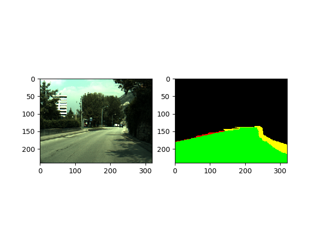
The green surface denotes True Positives, the red False Positives, the yellow False Negatives and the black True Negatives. The code for generating that, is in the calculate_metrics function above.
But what about more frames?
Scores in just one frame are not enough for us though. We would ideally want to recreate the numbers in the original paper, for the entire DIPLODOC sequence. Ideally, we would like the numbers to be close or identical to the paper, testing for, reproducibility (duh)!
For this, we will use the function road_detection.test_on_diplodoc(). Running it, will allow us to get a first glimpse of the result, even with the naive static seed selection method. Let’s fire up ipython (while inside the python directory):
$ ipython
Python 3.6.6 |Anaconda, Inc.| (default, Oct  9 2018, 12:34:16)
Type 'copyright', 'credits' or 'license' for more information
IPython 7.1.1 -- An enhanced Interactive Python. Type '?' for help.


In [1]: import road_detection


In [2]: m = road_detection.test_on_diplodoc()
F1=0.75: 100%|████████████████████████████| 450/450 [00:35<00:00, 12.55frames/s]
F1=0.94: 100%|████████████████████████████| 150/150 [00:11<00:00, 13.21frames/s]
F1=0.97: 100%|████████████████████████████| 100/100 [00:07<00:00, 13.56frames/s]
F1=0.81: 100%|██████████████████████████████| 60/60 [00:04<00:00, 13.41frames/s]
F1=0.98: 100%|████████████████████████████| 100/100 [00:07<00:00, 13.86frames/s]

In [3]: import numpy as np


In [4]: np.mean([mm['R'] for mm in m])
Out[4]: 0.9392746787161157


In [5]: np.mean([mm['P'] for mm in m])
Out[5]: 0.9462052090422761
In [3]: np.mean([mm['R'] for mm in m])
Not too bad to start with! A mean recall of 0.939 with mean precision of 0.946 are quite encouraging. The original -best performance- numbers from the paper were: mean recall (completeness in the paper) of 0.957 and mean precision (correctness in the paper) of 0.969.
We are still around 2% worse in both precision and recall. Getting closer to the targets and explaining the process will be the topic of Part 3. I will also try to compare with Matlab results and upload the code for that, for completeness. I will also discuss why we shouldn’t expect identical results and try to objectively compare Python and Matlab for research reproducibility and rapid prototyping.
–EDIT–
The numbers reported aboωe are actually even better. The ground truth parsing code did not take into account the occlusions from objects, hence using only the actual unobstructed road. When I fixed that, the new results were: Recall = 0.9568 and Precision = 0.9442. Happy days! only 2% of precision to go :)
As always, I will be very interested in comments and reporting of bugs in the code. After all, this is my first attempt of open-sourcing my research, so there probably are a lot of issues to be found.